Analytics gallery¶

Exhibits of stochvolmodels. Software citation: CITATION.cff.

Every figure in the documentation is listed here with the question it answers, the data behind it and the code that produces it. Each figure belongs to one of four classes, and its caption says which:

Class	What it is
Paper replication	A published figure regenerated offline by calling the paper’s own module with the paper’s parameters
Paper reproduction	A crop of a figure of the open-access IJTAF article, under CC BY 4.0, where the inputs cannot be distributed
Historical snapshot	Computed from an option chain bundled with the package, with its quote date
Synthetic teaching exhibit	Drawn from a page’s canonical script with fixed parameters and seed

Conventions¶

Item	Convention
Measure	The money-market-account (MMA) measure unless a caption names another: the inverse measure, or the annuity and forward measures of the rates exhibits
Volatility	Annualised; implied volatilities are Black-Scholes-Merton, except in the rates exhibits, which show normal volatilities in basis points
Monte Carlo	Seeded; the number of paths, the steps per year and the seed are in the caption and the registry
Error measure	Root-mean-square difference of implied volatilities, labelled “mse” in the package’s plot legends
One calculation	A figure’s tables and the numbers its article quotes come from the same functions of the page’s canonical script
Provenance	`analytics_manifest.json` records the configuration, the source commit and hashes, the package versions, the numerical checks and the image hashes

Regenerate every exhibit into a new directory outside the checkout, validate it, and verify the committed previews against the manifest:

python -m scripts.docs_analytics.run --all --output-root <new directory outside the checkout>
python -m scripts.docs_analytics.validate --run-root <that directory>
python -m scripts.docs_analytics.run --verify

The registry is scripts/docs_analytics/registry.json.

The log-normal SV model¶

Drift and paths of volatility¶


Question	How does the quadratic drift pull high volatility back faster, and what does that do to the paths of volatility?
Class	Synthetic teaching exhibit; panels A and B drawn by the paper module `vol_drift.py`
Parameters	\(\kappa_1 = 4\), \(\theta = 1\), \(\vartheta = 1.75\), \(\kappa_2 = 0, 4, 8\); 20,000 daily paths over one year with common increments, seed 7
Result	The 99th percentile of one-year volatility falls from 3.94 to 1.91 as \(\kappa_2\) rises from 0 to 8
Script	`examples/docs/logsv_model.py`
Producer	`scripts/docs_analytics/logsv_model.py`, `produce_logsv_drift_and_paths`
Article	Log-normal stochastic volatility model with quadratic drift

Steady-state distribution of volatility¶


Question	How does the quadratic mean reversion shape the steady-state density of volatility, its skewness and the kurtosis of returns?
Class	Paper replication, IJTAF Fig. 1
Parameters	\(\theta = 1\), \(\vartheta = 1.5\); density for \(\kappa_1 = 4\) and \(\kappa_2 = 0, 4, 8\); skewness and kurtosis for \(\kappa_1 = 1, 4, 8\)
Result	Excess kurtosis of returns 28.5, 2.05 and 1.26 for \(\kappa_2 = 0, 4, 8\) with \(\kappa_1 = 4\)
Paper module	`papers/logsv_model_with_quadratic_drift/steady_state_pdf.py`
Producer	`scripts/docs_analytics/logsv_model.py`, `produce_steady_state_density`
Article	Steady-state distribution, moments and expected QV

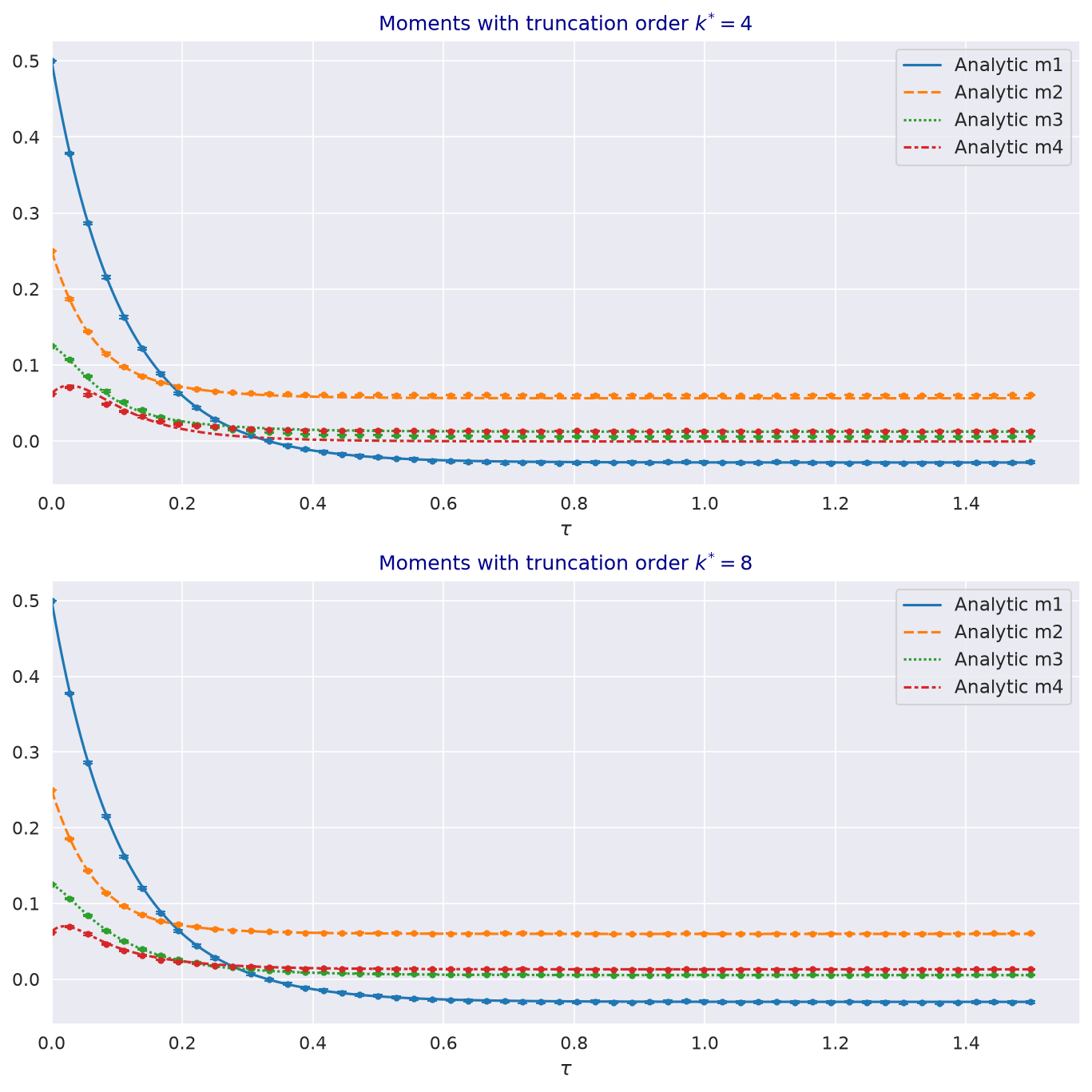
Moments of volatility against Monte Carlo¶


Question	How accurate is the truncated moment system at orders four and eight against Monte Carlo simulation?
Class	Paper replication, IJTAF Fig. 2
Parameters	\(\sigma_0 = 1.5\), \(\theta = 1\), \(\kappa_1 = \kappa_2 = 4\), \(\vartheta = 1\); 100,000 paths, seed 37
Result	At long horizons, order eight matches the stationary moments within 0.2%, order four within 6%
Paper module	`papers/logsv_model_with_quadratic_drift/moments_vol_qvar.py`
Producer	`scripts/docs_analytics/logsv_model.py`, `produce_vol_moments_vs_mc`
Article	Steady-state distribution, moments and expected QV

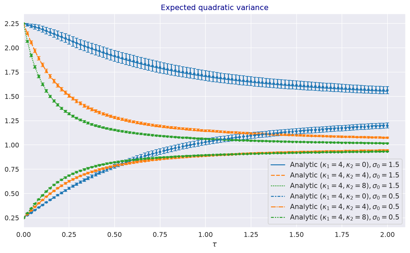
Expected quadratic variance against Monte Carlo¶


Question	How does the expected quadratic variance evolve from a high and a low initial volatility, and does the truncated system agree with simulation?
Class	Paper replication, IJTAF Fig. 3
Parameters	\(\kappa_1 = 4\), \(\kappa_2 = 0, 4, 8\), \(\theta = 1\), \(\vartheta = 1.5\), \(\sigma_0 = 1.5\) and 0.5; 25,000 paths (the paper used 100,000), seed 37
Result	From \(\sigma_0 = 1.5\), the two-year expected QV is 1.55, 1.07 and 1.02 for \(\kappa_2 = 0, 4, 8\)
Paper module	`papers/logsv_model_with_quadratic_drift/moments_vol_qvar.py`
Producer	`scripts/docs_analytics/logsv_model.py`, `produce_expected_qvar_vs_mc`
Article	Steady-state distribution, moments and expected QV

A Monte Carlo test of the martingale condition¶


Question	Does the simulated expected price stay at its initial value inside the region of Theorem 3.7 and fall below it outside?
Class	Synthetic teaching exhibit
Parameters	\(\kappa_2 = 0\) and 1, \(\beta\) from -1 to 1.4, \(\kappa_1 = 2\), \(\theta = \sigma_0 = 1\), \(\vartheta = 1.5\); 200,000 paths per point, seed 5
Result	Well outside the region the one-year expected price falls to about 0.80 of its initial value
Script	`examples/docs/martingale_conditions_and_skews.py`
Producer	`scripts/docs_analytics/logsv_model.py`, `produce_martingale_test`
Article	Martingale conditions, measures and positive skews

Smiles and the sign of the volatility beta¶


Question	How does the sign of the volatility beta set the direction of the implied volatility skew?
Class	Synthetic teaching exhibit
Parameters	\(\beta\) from -1 to 1, \(\sigma_0 = \theta = 0.5\), \(\kappa_1 = 2\), \(\kappa_2 = 2.5\), \(\vartheta = 1.5\); one month
Result	The difference between the implied volatilities at strikes 1.2 and 0.8 goes from -0.174 to 0.168
Script	`examples/docs/martingale_conditions_and_skews.py`
Producer	`scripts/docs_analytics/logsv_model.py`, `produce_smiles_in_beta`
Article	Martingale conditions, measures and positive skews

Transform pricing¶

First-order expansion coefficients¶


Question	How do the first-order expansion coefficients and the leading term evolve with maturity?
Class	Paper replication, IJTAF Fig. 4
Parameters	\(\Phi = -0.5 + 2i\), MMA measure; \(\sigma_0 = 0.8327\), \(\theta = 1.0139\), \(\kappa_1 = 4.8606\), \(\kappa_2 = 4.7938\), \(\beta = 0.1985\), \(\varepsilon = 2.369\), those of the paper’s figure code (the caption cites Eq. (6.4))
Result	\(A^{(0)}(1) = -1.8986 + 0.1060i\) and \(E^{[1]}(1) = 0.1593 + 0.0163i\)
Paper module	`papers/logsv_model_with_quadratic_drift/ode_sol_in_time.py`
Producer	`scripts/docs_analytics/transforms.py`, `produce_expansion_odes`
Article	The moment generating function and its affine expansion

Second-order expansion coefficients¶


Question	How do the second-order expansion coefficients evolve, and how small are the higher coefficients?
Class	Paper replication, IJTAF Fig. 5
Parameters	As for Fig. 4
Result	\(A^{(2)}\), \(A^{(3)}\) and \(A^{(4)}\) stay below \(10^{-4}\) at one year; \(E^{[2]}(1) = 0.1589 + 0.0162i\)
Paper module	`papers/logsv_model_with_quadratic_drift/ode_sol_in_time.py`
Producer	`scripts/docs_analytics/transforms.py`, `produce_expansion_odes`
Article	The moment generating function and its affine expansion

Densities from the expansion against Monte Carlo¶


Question	How close are the densities from the first- and second-order expansions to simulation?
Class	Paper replication, IJTAF Fig. 6, computed with the package because the paper module needs `qis`
Parameters	One month; Eq. (6.4) with the vol-of-vol scaled by 0.6, as the paper’s figure code; 400,000 paths with daily steps, seed 37
Result	The log-return densities differ from the histogram by 0.0138 and 0.0125 in total absolute probability, about the sampling noise of 0.0127
Script	`examples/docs/affine_expansion.py`
Producer	`scripts/docs_analytics/transforms.py`, `produce_expansion_pdfs_vs_mc`
Article	The moment generating function and its affine expansion

Fourier prices against Black-Scholes¶


Question	Does the Fourier pricer reproduce Black-Scholes at zero vol-of-vol, and how does the error fall with the grid?
Class	Synthetic teaching exhibit
Parameters	Zero vol-of-vol, \(\sigma_0 = \theta = 0.4\); one week, one month and one year; 100 to 2,000 grid points
Result	At the default 1,000 points the largest price error is \(1.3 \times 10^{-7}\) at one week and below \(2 \times 10^{-10}\) at one month and one year
Script	`examples/docs/european_option_pricing.py`
Producer	`scripts/docs_analytics/transforms.py`, `produce_fourier_vs_bsm`
Article	Fourier pricing of European options

Net delta of inverse options¶


Question	How does the net delta of an inverse option differ from its Black delta?
Class	Synthetic teaching exhibit; the computation of `papers/inverse_options/compare_net_delta.py`
Parameters	One week, 60% volatility, strike 50,000 dollars
Result	At the money, the call’s Black delta 0.5166 against a net delta of 0.4834, and the put’s -0.4834 against -0.5166
Script	`examples/docs/inverse_options.py`
Producer	`scripts/docs_analytics/transforms.py`, `produce_inverse_net_delta`
Article	Inverse options and the inverse measure

Options on quadratic variance¶


Question	What skew do call options on quadratic variance have, and do the MMA and inverse valuations agree with simulation?
Class	Paper replication, IJTAF Fig. 10, computed with the package because the paper module needs `qis`
Parameters	Eq. (6.4); packaged QV chain with strikes from 75% to 150% of the expected QV; 400,000 paths with 5,760 steps per year, seed 13 (the paper: 200,000 paths, the pricer’s default steps)
Result	Upward skews, from 344% to 368% at one week; MMA and inverse within \(5 \times 10^{-4}\); every strike inside the 95% Monte Carlo interval
Script	`examples/docs/quadratic_variance_options.py`
Producer	`scripts/docs_analytics/transforms.py`, `produce_qvar_option_smiles`
Article	Expected quadratic variance, variance swaps and QV options

Simulation and validation¶

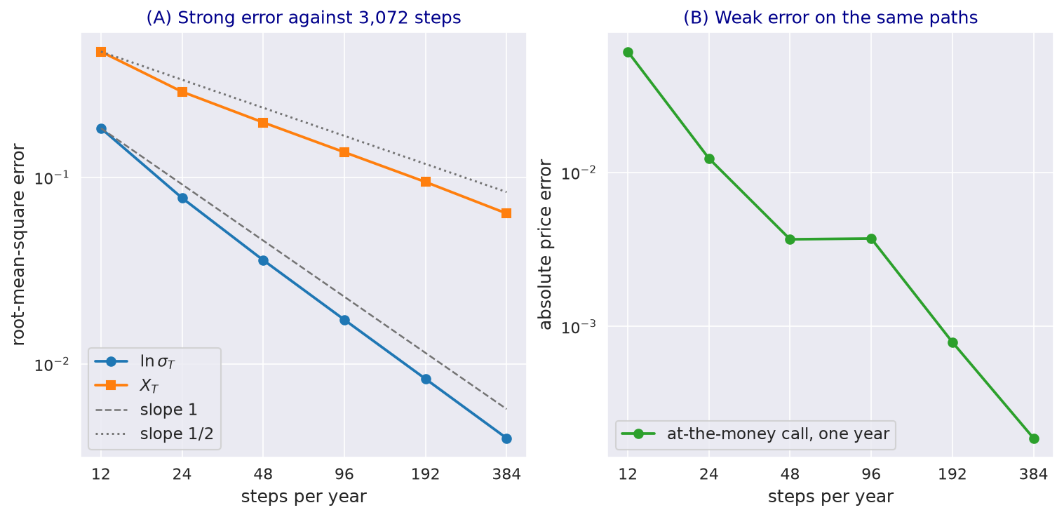
Convergence of the simulation scheme¶


Question	How do the strong and weak errors of the simulation scheme fall with the time step?
Class	Synthetic teaching exhibit
Parameters	`LOGSV_BTC_PARAMS`, one year, 12 to 384 steps against 3,072 on the same Brownian paths; 20,000 paths, seed 3
Result	The error of \(\ln \sigma_T\) falls from 0.1835 to 0.0040, order about one; that of \(X_T\) with order about one half
Script	`examples/docs/monte_carlo_simulation.py`
Producer	`scripts/docs_analytics/logsv_model.py`, `produce_mc_convergence`
Article	Monte Carlo simulation schemes

Transform against Monte Carlo on the Bitcoin chain¶


Question	Where on the smile do transform and Monte Carlo implied volatilities separate?
Class	Historical snapshot: maturities and forwards of the Bitcoin chain of 21 October 2021
Parameters	The case study’s fit; 33 strikes within four standard deviations; 400,000 paths, 1,440 steps per year, seed 7
Result	Every strike inside the 95% interval up to two months; 3 of 33 at 0.43 years, where the transform is above the simulation in the wings
Script	`examples/docs/analytic_vs_monte_carlo.py`
Producer	`scripts/docs_analytics/transforms.py`, `produce_analytic_vs_mc_btc`
Article	Analytic versus Monte Carlo validation

Calibration¶

Profiles of the calibration objective¶


Question	How sharply does the calibration objective identify each fitted parameter?
Class	Historical snapshot: Bitcoin implied volatilities of 21 October 2021
Parameters	The case study’s fit; one parameter moved at a time
Result	A 10% change multiplies the objective by about 33 for \(\sigma_0\), 9.5 for \(\theta\) and 1.3 for \(\varepsilon\); a change of 0.1 in \(\beta\) doubles it
Script	`examples/docs/calibration.py`
Producer	`scripts/docs_analytics/calibration.py`, `produce_calibration_objective_profiles`
Article	Calibration to implied volatilities

The approximate smile fitter¶


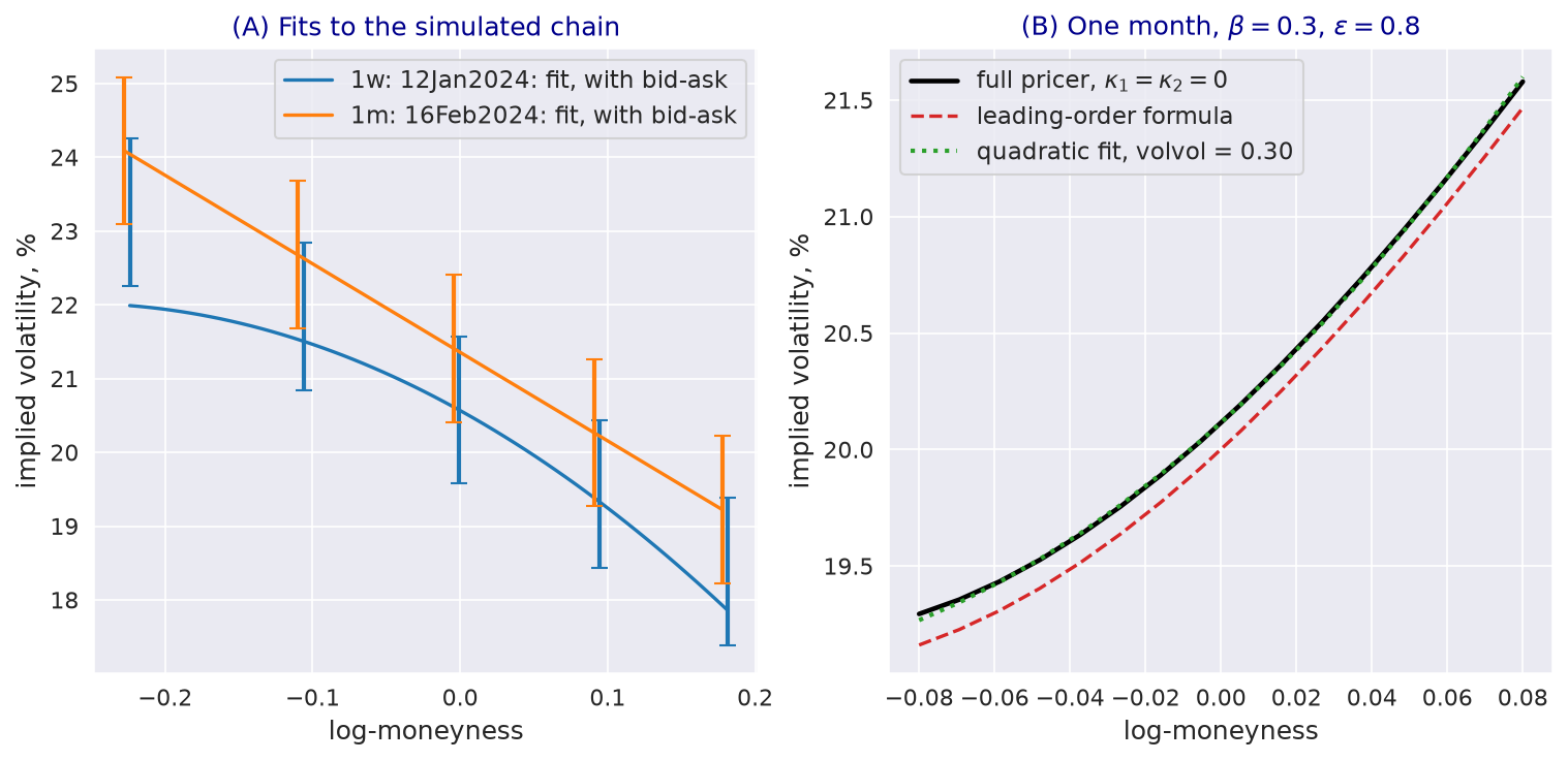
Question	How close is the approximate smile fitter to the full model?
Class	Synthetic teaching exhibit: a generated chain and a model smile
Parameters	`get_oca_simulated_chain_data`; one-month model smile with \(\sigma_0 = 0.2\), \(\beta = 0.3\), \(\varepsilon = 0.8\) and no mean reversion
Result	The leading-order formula within 0.15 volatility points of the full pricer; the quadratic fit within 0.05 points, with its own vol-of-vol of 0.30
Script	`examples/docs/logsv_smile_fitter.py`
Producer	`scripts/docs_analytics/calibration.py`, `produce_smile_fitter_fit`
Article	Approximate log-normal SV smile fitter

Other models¶

Heston against the log-normal SV model¶


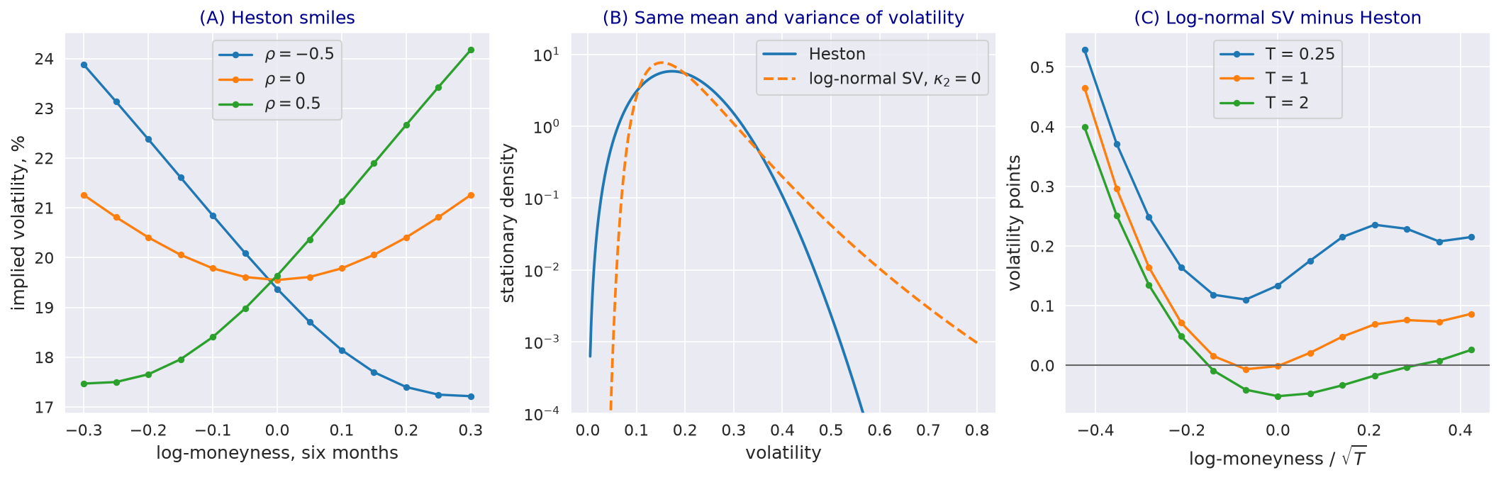
Question	How do the two models differ in volatility distribution and in smile at matched dynamics?
Class	Synthetic teaching exhibit
Parameters	Heston \(V_0 = \theta = 0.04\), \(\kappa = 4\), \(\vartheta = 0.4\); a log-normal SV model with the same initial volatility, correlation and stationary mean and variance of volatility
Result	Volatility above 50% with probability 0.005% under Heston and 0.31% under the log-normal SV model; smiles equal at the money at one and two years
Script	`examples/docs/heston_model.py`
Producer	`scripts/docs_analytics/other_models.py`, `produce_heston_vs_logsv`
Article	The Heston model as a benchmark

Smiles of clustered jumps¶


Question	What smile does jump clustering produce at the same mean jump intensity?
Class	Synthetic teaching exhibit
Parameters	`HawkesJDParams` defaults, self-excitation with branching ratios 0, 0.35 and 0.7; 200,000 paths, seed 2026
Result	Clustering lowers the at-the-money volatility and lifts the wings; the simulation separates from the transform at six months for the strongest clustering
Script	`examples/docs/hawkes_jump_diffusion.py`
Producer	`scripts/docs_analytics/other_models.py`, `produce_hawkes_smiles`
Article	Jump-diffusion with clustered jumps

Mixture and Student-t smiles¶


Question	What smiles can mixtures and Student-t laws produce without dynamics?
Class	Synthetic teaching exhibit
Parameters	Six months, forward 100; mixtures of two to four states; Student-t with \(\nu\) of 3, 5 and 30 and 20% volatility at the forward
Result	Closed forms equal numerical integration to \(10^{-12}\); more mixture states steepen the put wing; small \(\nu\) curves both wings
Script	`examples/docs/terminal_distribution_models.py`
Producer	`scripts/docs_analytics/other_models.py`, `produce_terminal_distribution_smiles`
Article	Gaussian-mixture and Student-t smiles

Swaption skews and the volatility beta¶


Question	How does the volatility beta shape swaption skews?
Class	Synthetic teaching exhibit
Parameters	RDR Table 2 base scenario with the betas multiplied by \(-2\), 0 and 1; 2y expiry; 20,000 paths, seed 16
Result	Symmetric smile without a beta, skew in the direction of its sign; the base scenario inside the Monte Carlo interval at all 21 strikes
Script	`examples/docs/factor_hjm_stochastic_volatility.py`
Producer	`scripts/docs_analytics/rates.py`, `produce_fhjm_swaption_skews`
Article	Stochastic volatility for factor HJM rates

Applications¶

Weekly calibrations to Bitcoin options, 2019 to 2023¶


Question	How well did weekly calibrations fit Bitcoin options, and how did the fitted parameters move?
Class	Paper reproduction, IJTAF Fig. 7, CC BY 4.0; cropped, sub-captions removed
Data	Deribit Bitcoin options, weekly, April 2019 to October 2023; not distributable
Result	Average model error 1.59 volatility points against an average bid-ask spread of 2.30
Producer	`scripts/docs_analytics/paper_pdf.py`, `produce_pdf_crop`, page 45 of the article PDF
Article	Bitcoin options: MMA, inverse and QV valuation

A Bitcoin fit on one day¶


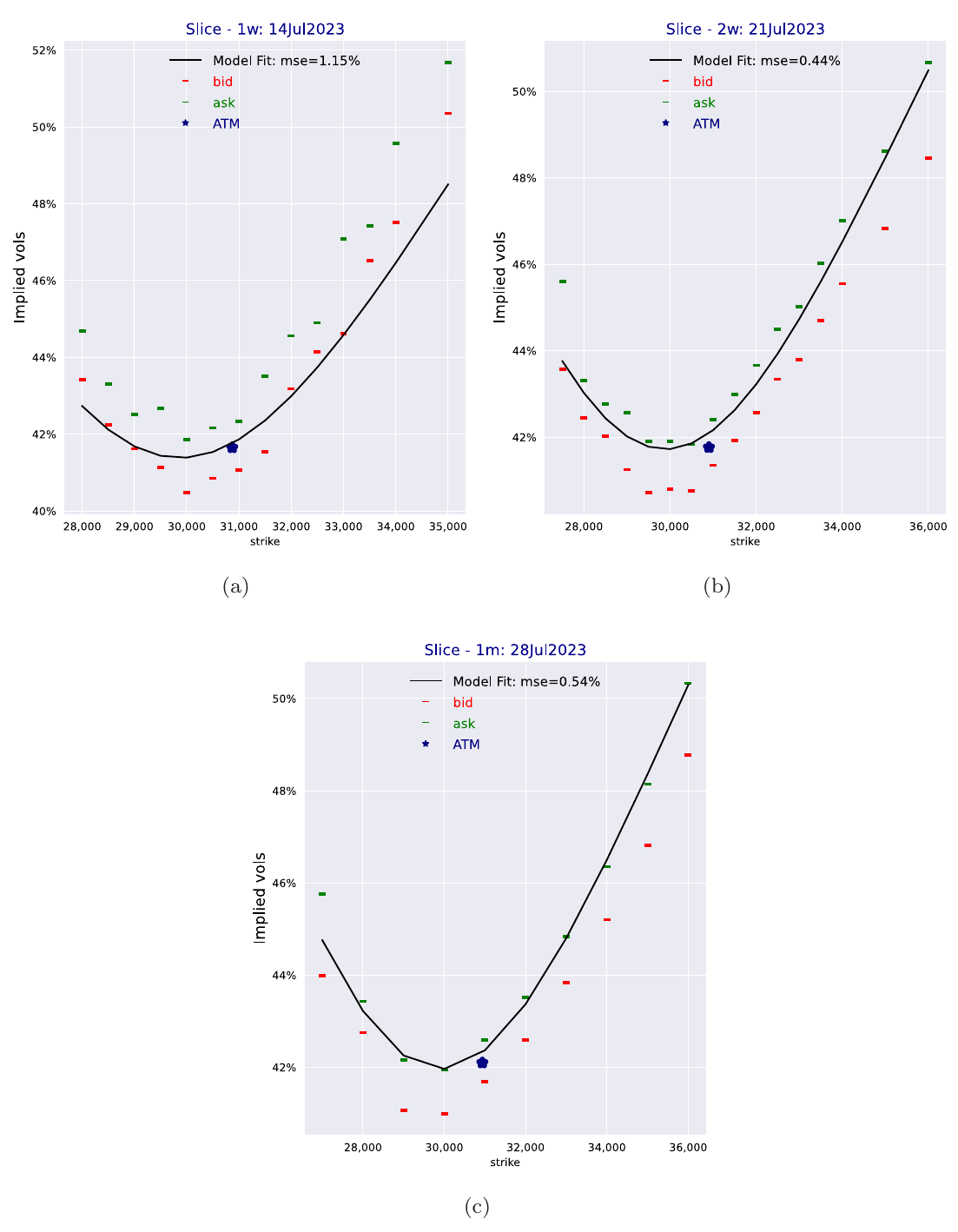
Question	How closely does the calibrated model match the bid and ask quotes of the three most liquid expiries?
Class	Paper reproduction, IJTAF Fig. 8, CC BY 4.0; cropped
Data	Deribit Bitcoin options; not distributable
Parameters	Eq. (6.4): \(\sigma_0 = 0.41\), \(\theta = 0.38\), \(\beta = 0.50\), \(\varepsilon = 3.06\), \(\kappa_1 = 2.21\), \(\kappa_2 = 2.18\)
Producer	`scripts/docs_analytics/paper_pdf.py`, `produce_pdf_crop`, page 47 of the article PDF
Article	Bitcoin options: MMA, inverse and QV valuation

The paper’s configuration on the bundled Bitcoin chain¶


Question	Does the paper’s calibration configuration fit the bundled Bitcoin chain within its bid-ask spread?
Class	Historical snapshot: Bitcoin implied volatilities of 21 October 2021
Parameters	`FITTED` of the canonical script: \(\sigma_0 = 0.863\), \(\theta = 1.04\), \(\beta = 0.130\), \(\varepsilon = 1.63\)
Result	Error inside the average spread for three of the four expiries
Script	`examples/docs/app_bitcoin_options.py`
Producer	`scripts/docs_analytics/calibration.py`, `produce_btc_case_fit`
Articles	Bitcoin options: MMA, inverse and QV valuation, Calibration to implied volatilities

MMA and inverse valuation against Monte Carlo¶


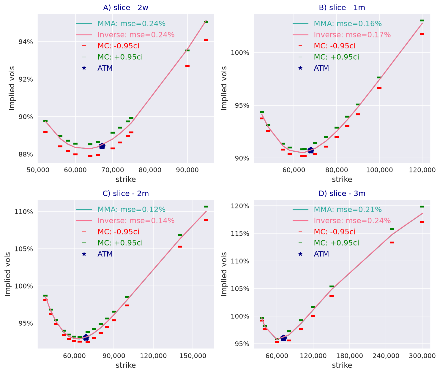
Question	Do the MMA and inverse valuations agree with each other and with Monte Carlo simulation on the bundled chain?
Class	Historical snapshot: Bitcoin implied volatilities of 21 October 2021
Parameters	`FITTED`; 400,000 paths, 360 steps per year, seed 7
Result	Valuations within \(10^{-4}\) of the forward of each other; Monte Carlo within two standard errors in the script’s check
Script	`examples/docs/app_bitcoin_options.py`
Producer	`scripts/docs_analytics/calibration.py`, `produce_btc_case_measures`
Articles	Bitcoin options: MMA, inverse and QV valuation, Inverse options and the inverse measure

One model on five underlyings¶


Question	Does one parameterisation fit equity, VIX, gold and inverse-ETF skews?
Class	Historical snapshots: SPY, GLD, SQQQ and VIX of 15 July 2022; Bitcoin of 21 October 2021
Parameters	`FITTED` of the canonical script, recorded in `papers/logsv_model_with_quadratic_drift/calibrations.py`; the two-month maturity
Result	\(\beta\) negative for SPY only; every fit satisfies \(\kappa_2 \ge 2 \beta\)
Script	`examples/docs/app_positive_and_negative_skews.py`
Producer	`scripts/docs_analytics/calibration.py`, `produce_cross_asset_calibrations`
Article	One model for equity, VIX, gold and leveraged-ETF skews

USD swaption fit¶


Question	Does one set of parameters per expiry fit the swaption smiles of three tenors?
Class	Paper replication, RDR Fig. 5, regenerated from `papers/sv_for_factor_hjm/calibration_fig_5_6_7.py` with the module’s parameters, which differ from the published tables
Parameters	USD swaptions of 18 August 2023, expiries 1y to 5y, tenors 2y, 5y, 10y; first-order expansion
Result	Root-mean-square error 1.15, 0.48 and 0.70 bp by tenor; 2.29, 1.38 and 1.95 bp with Table 1
Script	`examples/docs/app_swaptions_and_sofr_options.py`
Producer	`scripts/docs_analytics/rates.py`, `produce_rdr_fig5_swaption_fit`
Article	USD swaptions and SOFR futures options

Swaptions against Monte Carlo at 5y¶


Question	Is the first-order expansion accurate against Monte Carlo at the 5y expiry?
Class	Paper replication, RDR Fig. 6, regenerated from `papers/sv_for_factor_hjm/calibration_fig_5_6_7.py` with the module’s parameters, which differ from the published tables
Parameters	5y expiry; 200,000 paths in 20 batches, seeds 1 to 20
Result	Inside the 95% interval at 19, 15 and 0 of 21 strikes; 0.55 to 1.46 bp above it for the 10y tenor
Script	`examples/docs/app_swaptions_and_sofr_options.py`
Producer	`scripts/docs_analytics/rates.py`, `produce_rdr_fig6_swaption_mc`
Article	USD swaptions and SOFR futures options

Swaptions under parameter shocks¶


Question	Does the first-order expansion stay accurate under the parameter shocks of Table 2?
Class	Paper replication, RDR Fig. 7, regenerated from `papers/sv_for_factor_hjm/calibration_fig_5_6_7.py` with the module’s parameters, which differ from the published tables
Parameters	The four scenarios of Table 2; 2y expiry; 200,000 paths per scenario
Result	All 63 strikes inside for the base and level-shifted scenarios; 9 to 11 and 7 to 9 of 21 per tenor with vol-of-vol times 4 and betas times \(-2\)
Script	`examples/docs/app_swaptions_and_sofr_options.py`
Producer	`scripts/docs_analytics/rates.py`, `produce_rdr_fig7_shock_scenarios`
Article	USD swaptions and SOFR futures options

SOFR futures option fit¶


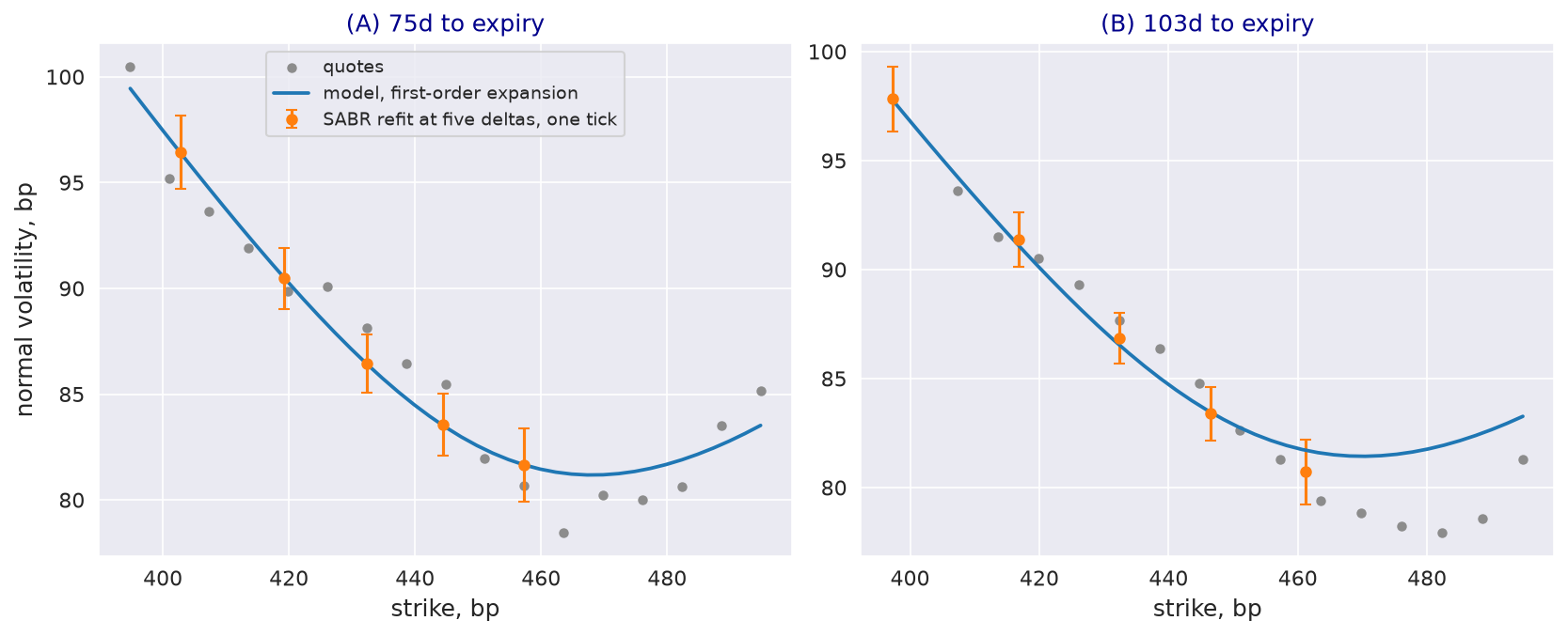
Question	Does the model fit the smiles of short-dated SOFR futures options?
Class	Paper replication, RDR Fig. 8, regenerated from `papers/sv_for_factor_hjm/calibration_fig_8_9.py` with the module’s parameters, which differ from the published tables
Parameters	3M SOFR options at 75 and 103 days, SABR refit at five deltas; first-order expansion
Result	Root-mean-square error 0.03 and 0.48 bp against the refit, inside one tick at every strike; 18.84 and 12.33 bp with Table 3
Script	`examples/docs/app_swaptions_and_sofr_options.py`
Producer	`scripts/docs_analytics/rates.py`, `produce_rdr_fig8_sofr_fit`
Article	USD swaptions and SOFR futures options

SOFR options against Monte Carlo¶


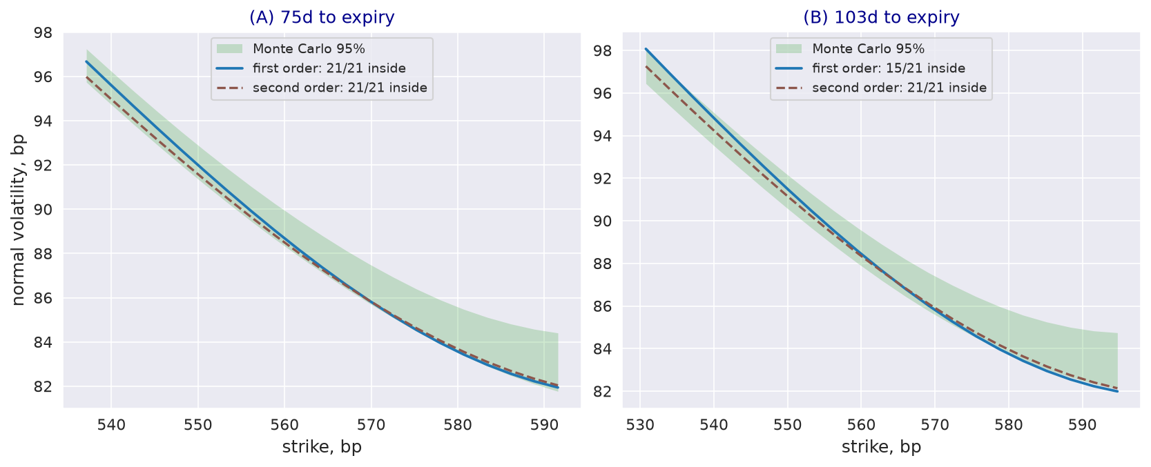
Question	Are the first- and second-order expansions accurate against Monte Carlo for SOFR options?
Class	Paper replication, RDR Fig. 9, regenerated from `papers/sv_for_factor_hjm/calibration_fig_8_9.py` with the module’s parameters, which differ from the published tables
Parameters	\(2^{17}\) paths, seed 20; strikes re-centred on the model futures rate
Result	At 75 days both orders inside at 21 of 21 strikes; at 103 days 15 and 21 of 21
Script	`examples/docs/app_swaptions_and_sofr_options.py`
Producer	`scripts/docs_analytics/rates.py`, `produce_rdr_fig9_sofr_mc`
Article	USD swaptions and SOFR futures options

Impermanent loss and its replication¶


Question	Do European payoffs replicate the impermanent loss, and how does its value depend on vol-of-vol?
Class	Synthetic teaching exhibit
Parameters	`PARAMS` of the canonical script, the example of `papers/il_hedging/run_logsv_for_il_payoff.py`: range 2,000 to 2,400 around 2,200, ten days
Result	Replication exact to \(10^{-12}\); expected loss 1.650% of the position at \(\varepsilon = 1\) and 1.786% at \(\varepsilon = 4\)
Script	`examples/docs/app_impermanent_loss_hedging.py`
Producer	`scripts/docs_analytics/applications.py`, `produce_il_replication`
Article	Hedging impermanent loss with the LogSV MGF

Persistence and stationary laws of four volatility indices¶


Question	What persistence and stationary distribution do the recorded parameters imply for four volatility indices?
Class	Synthetic teaching exhibit: parameters recorded in `papers/volatility_models/article_figures.py`, no market data
Parameters	VIX, MOVE, OVX and Bitcoin; 50,000 paths from stationary starts, seed 7
Result	Half-lives of 108, 380, 50 and 48 business days; right-skewed laws with similar dispersion of log-volatility
Script	`examples/docs/app_robust_volatility_models.py`
Producer	`scripts/docs_analytics/other_models.py`, `produce_robust_vol_models`
Article	What makes a stochastic volatility model robust